Unlocking the power of Biquad Filters
Infinite Impulse Response (IIR) filters or recursive linear filters normally require less computing resources than a Finite Impulse Response (FIR) filter of similar performance. If low computational complexity is important, e.g. because of speed or power constraints, then IIR may be a good option. Moreover, the group delay of IIR filters is typically smaller, since IIR filters allow to meet a set of design specifications with a far smaller filter order compared to FIR. Sometimes, reduced group delay is preferred to achieve a shorter filter transient response, allowing to quickly react to changes in a signal.
Drawbacks of IIR filters include its non-linear phase response, i.e. the group delay depends on frequency, as well as the danger of instability, which is an inherent aspect of using feedback. High-order IIR filters can be highly sensitive to quantization of their coefficients, and can easily become unstable. This is much less of a problem with first and second-order filters. Second order IIR filters are often called biquads and a common implementation of higher order filters is to cascade biquads, to ensure stability.In this blog, we will look into a practical approach towards the use of biquad filters.
Definition
A digital biquad filter is a second-order IIR filter, containing two poles and two zeros. Biquadratic or biquad refers to the fact that its transfer function is the ratio of two quadratic functions:
$$ H(z) = \frac{b_0+b_1 z^{-1}+b_2 z^{-2}} {a_0+a_1 z^{-1}+a_2 z^{-2} } . $$ Typically, the denominator coefficients are normalized such that \(a_0 = 1\), $$ H(z) = \frac{b_0+b_1 z^{-1}+b_2 z^{-2}} {1+a_1 z^{-1}+a_2 z^{-2} } . $$ Sometimes also the numerator coefficients are normalized such that \(b_0 = 1\), $$ H(z) = g \frac{1+b_1 z^{-1}+b_2 z^{-2}} {1+a_1 z^{-1}+a_2 z^{-2} } , $$ where the gain \( g \) is introduced.
Two quadratic equations
Real second-order polynomials have complex roots, therefore the poles come in complex conjugated pairs. We can distill the essence of these polynomials into something elegant and insightful—a simple expression that revolves around two key parameters: the radius \(R\) and angle \( \theta\) of the positive-frequency pole, i.e. $$ \begin{array}{ll} A(z) & = (1-R e^{j\theta} z^{-1})(1-R e^{-j\theta} z^{-1}) \cr & = 1-2 R \cos{\theta}z^{-1} + R^2 z^{-2} , \end{array} $$ since \(\cos{x} = (e^{+jx} +e^{-jx})/2 \). So, in this case the denominator coefficients become: $$ \begin{array}{ll} a_1 & = - 2 R \cos{\theta} \cr a_2 & = R^2 . \end{array} $$ Resonance occurs at the positive-frequency pole, i.e. at \(\theta = 2 \pi f_r T_s [\text{rad}]\), where \(f_r [\text{Hz}]\) is the resonance frequency, and \( T_s [\text{s}] \) is the sampling period. The distance of the pole to the origin of the z-plane, i.e. the pole-radius \(R\), determines the quality of resonance. The quality factor \(Q\) of the resonator may be thought of as the number of cycles of oscillation at the resonant frequency in the impulse response before it substantially decays to zero. When \(R \approx 1\), a reasonable definition of the 3dB-bandwidth is \( BW \approx \ln{R}/\pi T_s [\text{Hz}] \).
If the two zeroes form a complex conjugated pair as well, then the numerator can represented in a similar fashion, i.e. in terms of a zero-angle and radius. Now, the zero-angle determines the so-called anti-resonance frequency, or notch frequency. Likewise, the zero-radius affects the depth and width of the notch. More often, when creating a resonator, one zero is placed at DC (\(z = 1\)), and the other at the Nyquist frequency (\(z = -1\)), such that \(b_1 = 0\) and \(b_2 = -1 \). Now the numerator polynomial equals $$ B(z)=1-z^{-2}=(1+z^{-1})(1-z^{-1}). $$
Since there is an obvious relation between the biquad coefficients and its resonance frequency and quality factor, we can build a digital resonator that can be tuned on the fly. This useful tool is easily implemented on e.g. a microcontroller, as we will see further on.
Example
Consider a biquad filter operated at \(f_s = 8 [\text{kHz}]\) with transfer function $$ H(z) = \frac{1+\frac{1}{2}z^{-1}-\frac{1}{2}z^{-2}}{1-z^{-1}+\frac{1}{2}z^{-2}} = \frac{z^2+\frac{1}{2}z-\frac{1}{2}}{z^2-z+\frac{1}{2}}. $$
The poles of the system are found by finding the roots of the denominator, i.e. $$ p_{1,2} = \frac{1} {2} \pm \frac{1} {2} j , $$ which implies that the pole angle equals $$ \theta = \arctan{\frac{\frac{1} {2}}{\frac{1} {2}}} = \frac{\pi} {4} \text{rad}. $$ Given the sampling frequency, \(f_s = 8 \text{kHz} \), the resonance frequency equals $$ f_r = \frac {\theta} {2\pi T_s} = \frac {\pi/4} {2\pi T_s} = \frac {f_s}{8} = 1 \text{kHz} $$
Although it is not hard to compute poles and zeroes, typically a software tool is used. Here, we apply the signal processing module of the Python package SciPy, which is an open-source software for mathematics, science, and engineering available for the Python programming language, see scipy.signal.
First, we are going to specify the filter's numerator and denominator polynomials stacked in a single row vector. In order to properly define a row vector, we need a function from the Numpy package to create an array. NumPy is the fundamental package for scientific computing in Python.
Next, the zeroes, poles and gain are computed.
Matplotlib is used to vizualize the poles and zeroes in the complex z-plane.
import matplotlib.pyplot as plt

fig0, ax0 = plt.subplots()
ax0.grid(True)
ax0.set_title("Pole-zero plot")
ax0.set_xlim(-1.5, 1.5)
ax0.set_ylim(-1.25, 1.25)
ax0.set_xlabel('real')
ax0.set_ylabel('imaginary')
ax0.plot(z.real, z.imag, 'bo', fillstyle='none', ms = 10)
ax0.plot(p.real, p.imag, 'bx', fillstyle='none', ms = 10)
Let's indicate the unit circle as well as the real and imaginary axes in dashed lines.
from matplotlib import patches

unit_circle = patches.Circle((0,0), radius=1, fill=False, color='black', ls='--')
ax0.add_patch(unit_circle)
ax0.axvline(0, color='black', linestyle='--')
ax0.axhline(0, color='black', linestyle='--')
Finally, we need to actually show the figure.
In the pole-zero plot we can clearly see 2 zeroes and the complex-conjugated pole pair composing the biquad filter.

Design methods
Typically, the design of digital IIR filters is based on analog filters with feedback. Transfer functions of analog filters have been extensively studied and optimized for their amplitude and phase characteristics. These continuous-time filters can be described in the Laplace domain and can be transferred to discrete-time filters whose transfer functions are expressed in the z-domain, through the use of certain mathematical techniques such as the bilinear transform, impulse invariance, or pole–zero matching.
In practice, one would almost never apply such techniques manually, but rely on design tools that automate the computations. One such a tool is the signal processing module of the SciPy open-source software for mathematics, science, and engineering available for the Python programming language, see scipy.signal. Let's find out how to use SciPy to design biquad filters or biquad cascades.
Example
In this example, we are going to design a bandpass filter as a cascade of \( N \) biquad sections, a.k.a. second order sections (sos). This filter will be based on an analog template of a Butterworth filter. Note that while Butterworth filters have maximally flat pass and stopbands, this causes the transition band to be very wide.
First, we are going to specify some basic parameters, i.e. the sampling frequency, the pass band, and the number of biquads in the cascade.
f_s = 16000  # [Hz] sampling rate
f_pass = [90, 400]  # [Hz] pass band corner frequencies
N = 2  # number of biquad sections
Next, the Butterworth design method is invoked with the appropriate parameters.
from scipy import signal

sos = signal.butter(N=N, Wn=f_pass, btype='bandpass', output='sos', fs=f_s)
The resulting second-order sections matrix is a (N, 6) numpy.ndarray, where each row contains the coefficients of one biquad. So, sos[0, :] \( \triangleq [b_0, b_1, b_2, 1., a_1, a_2] \) is the vector of coefficients of the first biquad section. Typically, the numerator coefficients are normalized to \( b_0 \) except for the first section.
Now, let's determine the magnitude response of the filter.
f, H = signal.sosfreqz(sos, fs=f_s, worN=1024)

from numpy import log10, finfo
eps = finfo(float).eps
H_dB = 20 * log10(abs(H + eps))
Note that a small number eps is added to the modulus of the transfer function in order to suppress 'divide by zero' RuntimeWarning encountered in log10.
Again, Matplotlib is used to vizualize the filter response.
import matplotlib.pyplot as plt

fig0, ax0 = plt.subplots()
ax0.grid(True)
ax0.set_title("Frequency response")
ax0.set_xlim(f[1], f_s/2)
ax0.set_ylim(-40, 6)
ax0.set_xlabel('f[Hz]')
ax0.set_ylabel('Magnitude [dB]')
ax0.semilogx(f, H_dB, 'b')
ax0.axvline(f_pass[0], color='black', linestyle=':')
ax0.axvline(f_pass[1], color='black', linestyle=':')
ax0.axhline(-3, color='black', linestyle=':')
In the magnitude response plot, the corner frequencies are indicated by dashed vertical lines, showing -3dB damping w.r.t. the pass-band.

Likewise, the phase response of the filter is determined.
Note that the phase is not directly proportional to frequency; a property of IIR filters.

Let's further investigate the non-linear phase response by examining the group delay, i.e. the time delay of the amplitude envelopes of the various sinusoidal components of a signal. The group delay, \( \tau_g (f) \), is a measure of the slope of the phase response \( \phi(f) \) at a given frequency, i.e.
$$ \tau_g (f) = - \frac{1} {2 \pi} \frac{\partial \phi(f)} {\partial f} [\text{s}] $$
Let's compute the group delay of the filter.
When a signal is passed through the filter, all frequency components are delayed. In case of a non-linear phase response, the delay will be different for different frequencies.
fig2, ax2 = plt.subplots()
ax2.grid(True)
ax2.set_title("Group delay")
ax2.set_xlim(f[2], f_s/2)
ax2.set_ylim(0, 0.005)
ax2.set_xlabel('f[Hz]')
ax2.set_ylabel('Group delay [s]')
ax2.semilogx(f[1:], tau_g, 'b')
ax2.axvline(f_pass[0], color='black', linestyle='--')
ax2.axvline(f_pass[1], color='black', linestyle='--')
The delay variation means that signals consisting of multiple frequency components will suffer distortion because these components are not delayed by the same amount of time. At the expense of more computational complexity, a correction filter can be applied to make sure that all frequencies are delayed by the same amount, without much change to the magnitude response. This compensation method using an all-pas filter will be investigated further in another article.

In the example, the lowest frequencies passing the filter are delayed 4 times more than the highest frequencies! Considering that the sampling period equals \(T_s = 1/16000 \), the delay ranges from 16 samples for high frequencies to 64 samples for low frequencies.
Implementation
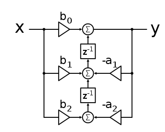
The most straightforward implementation of a biquad filter is the direct form 1 (DF1), which has the following difference equation: $$ y[n]= b_0 x[n] + b_1 x[n-1] + b_2 x[n-2] - a_1 y[n-1] - a_2 y[n-2]. $$ The DF1 implementation requires four delay registers. An equivalent circuit is the direct form 2 (DF2) implementation, which requires only two delay registers, or states. The DF2 implementation is called the canonical form, because it uses the minimal amount of states, adders and multipliers, yielding the same transfer function as the DF1 implementation. The difference equations for DF2 are: $$ \begin{array}{ll} y[n] &= b_0 w[n] + b_1 w[n-1] + b_2 w[n-2]) \cr w[n] &= x[n] - a_1 w[n-1] - a_2 w[n-2], \end{array} $$ where it assumed that \(a_0 = 1 \).
The transposed DF2 implementation is preferred over DF2, since the zeroes are implemented first, thus reducing possible explosion of internal states.
The difference equations for transposed DF2 are:
$$ \begin{array}{ll} y[n] &= b_0 x[n] + s_1[n-1] \cr s_1[n] &= s_2[n-1] + b_1 x[n] - a_1 y[n] \cr s_2[n] &= b_2 x[n] - a_2 y[n] . \end{array} $$
Sometimes, it useful to initialize a filter instead of starting from rest (empty registers). One way to construct initial conditions is to assume steady state, therefore \( n = n-1 \),
$$ \begin{array}{ll} y[n] &= b_0 x[n] + s_1[n] \cr &= b_0 x[n] + s_2[n] + b_1 x[n] - a_1 y[n] \cr &= b_0 x[n] + b_2 x[n] - a_2 y[n] + b_1 x[n] - a_1 y[n] \cr &= (b_0 + b_1 + b_2) x[n] - (a_1 + a_2) y[n] . \end{array} $$
So, first the steady state output to the initial input is computed from the DC gain \(H(0) \), $$ \begin{array}{ll} y[n] &= \frac{b_0 + b_1 + b_2} {1 + a_1 + a_2} x[n] \cr \cr &= H(0) x[n] . \end{array} $$
Then the registers are initialized,
$$ \begin{array}{ll} s_2[n] &= b_2 x[n] - a_2 y[n] \cr s_1[n] &= s_2[n] + b_1 x[n] - a_1 y[n] . \end{array} $$
Python implementation
Obviously, SciPy employs filtering functions such as signal.sosfilt that implement the difference equations. SciPy is mostly intended to work with stored data or blocks of data. Here we are going to compute the filter output to a sample stream, as opposed to block-processing or off-line processing. It is assumed that all necessary computations can be performed within a sample period, implying that an output sample comes available during the same sample period as the input was provided, which can be considered as real-time processing.
Let's first declare a Biquad class, where the constructor simply copies the coefficients to private class members,
class Biquad(object):

    def __init__(self, sos: list):
        super().__init__()
        if len(sos) != 6:
            raise ValueError('Invalid number of coefficients')
        self.b_0, self.b_1, self.b_2, self.a_0, self.a_1, self.a_2 = sos
        if self.a_0 != 1:
            raise ValueError('First feedback coefficient (a_0) is assumed to be equal to 1')
        self.s = 2*[0]
        self.initialized = False
The initialized flag is used to indicate whether the filter has been initialized.
Once initialized, the general difference equations apply.
The process() method implements DF2 to compute an output sample,
from math import isnan

def process(self, x: float) -> float:
    if x is None or isnan(x):
        return None
    if self.initialized:
        y = self.b_0 * x + self.s[0]
        self.s[0] = self.b_1 * x - self.a_1 * y + self.s[1]
        self.s[1] = self.b_2 * x - self.a_2 * y
    else:
        y = x * (self.b_0 + self.b_1 + self.b_2) / (1 + self.a_1 + self.a_2)
        self.s[1] = self.b_2 * x - self.a_2 * y
        self.s[0] = self.b_1 * x - self.a_1 * y + self.s[1]
        self.initialized = True
    return y
A cascade of biquad filters can now be defined as follows,
class Biquads(object):

    def __init__(self, sos: array):
        super().__init__()
        self.N = sos.shape[0]
        self.cascade = [Biquad(sos_) for sos_ in sos]

    def process(self, x: float) -> float:
        y = x
        for i in range(self.N):
            y = self.cascade[i].process(y)
        return y
As an example, compare the response of a low-pass biquad cascade to the sosfilt output.
from numpy import array, vectorize
from scipy import signal
import matplotlib.pyplot as plt

sos = signal.butter(N=5, Wn=250, btype='lowpass', output='sos', fs=1600)
biquad = Biquads(sos)

x = array([-1.0]*50 + [1.0]*50 + [0.0]*50)

f1 = signal.sosfilt(sos, x)
f2 = vectorize(biquad.process)(x)

fig0, ax0 = plt.subplots()
ax0.grid(True)
ax0.set_title("Filter response")
ax0.plot(x, 'k--', label='input')
ax0.plot(f1, 'b', alpha=0.5, linewidth=2, label='sosfilt')
ax0.plot(f2, 'r', alpha=0.25, linewidth=4, label='biquad')
ax0.set_xlabel('sample [#]')
ax0.legend(loc='best')

plt.show()
In the resulting plot you can check how the initialization of the biquad cascade differs from the sosfilt implementation.

C++ implementation
This sample-by-sample computation of a biquad cascade output is easily implemented in C++. Let's first declare a Biquad class with a process method, next to the constructor and destructor,
#include <vector>

class Biquad
{
    private:
    bool initialized = false;
    float a[3], b[3], s[2] = {0};

    public:
    Biquad(const std::vector<float>& sos);
    ~Biquad(){};

    float process(const float in);
};
The constructor simply copies the coefficients to private class members,
#include "biquad.h"
#include <stdexcept>
#include <vector>

Biquad::Biquad(const std::vector<float> &sos)
{
    if (sos.size() != 6)
        throw std::invalid_argument("Invalid number of coefficients");
    for (int i = 0; i < 3; i++) {
        b[i] = sos[i];
        a[i] = sos[i + 3];
    }
    if (a[0] != 1.0)
        throw std::invalid_argument("First feedback coefficient (a_0) is assumed to be equal to 1");
}
The process() method implements DF2 to compute an output sample,
float Biquad::process(const float in)
{
    float out;
    if (initialized)
    {
        out = b[0] * in + s[0];
        s[0] = s[1] + b[1] * in - a[1] * out;
        s[1] = b[2] * in - a[2] * out;
    }
    else
    {
        out = in * (b[0] + b[1] + b[2]) / (1 + a[1] + a[2]);
        s[1] = b[2] * in - a[2] * out;
        s[0] = s[1] + b[1] * in - a[1] * out;
        initialized = true;
    }
    return out;
}
A cascade of biquad filters can now be defined as follows,
class Biquads
{
    private:
    int nr_of_sections;
    std::vector<Biquad> cascade;

    public:
    Biquads(const std::vector<std::vector<float>> &sos);
    ~Biquads(){};

    float process(const float in);
};

Biquads::Biquads(const std::vector<std::vector<float>> &sos)
{
    nr_of_sections = sos.size();
    for (int i=0; i < nr_of_sections; i++)
        cascade.push_back(Biquad(sos[i]));
}

float Biquads::process(const float in)
{
     float out = in;

     for (int i=0; i < nr_of_sections; i++)
        out = cascade[i].process(out);

    return out;
}